English
 中文简体

A 50 Ω cable fitted with a 75 Ω connector will pass a continuity test, look perfectly assembled, and still ruin the link budget. That is why coaxial cable specifications deserve more attention than the jacket colour: the numbers describe behaviour a multimeter cannot see.
Coaxial cable specifications are the electrical and mechanical parameters that define how a cable behaves at a given frequency. Electrically that means characteristic impedance, attenuation, velocity factor, capacitance, power rating and maximum voltage. Mechanically it means conductor and dielectric dimensions, outer diameter, minimum bend radius, connector interface geometry and temperature limits.
The short answer: match impedance first, read attenuation at the frequency you will actually use, then confirm mechanical and interface limits. Everything else — capacitance, velocity factor, jacket rating — is a refinement that only matters once those three checks pass.
Content
- 1 The Electrical Specifications That Decide Whether a Link Works
- 2 Impedance, Connector Interfaces, and the Tolerance That Actually Matters
- 3 Mechanical Specifications and Installation Limits
- 4 Reading a Datasheet Without Being Misled
- 5 Matching Connectors, Adapters and Surge Protection
- 6 Frequently Asked Questions
- 7 A Short Checklist Before You Order
The Electrical Specifications That Decide Whether a Link Works
Four numbers carry most of the decision: impedance, attenuation, velocity factor and power rating. The rest of the datasheet supports them.
| Specification | Typical expression | What it controls | Common mistake |
|---|---|---|---|
| Characteristic impedance | 50 Ω or 75 Ω, often ±2 Ω | Reflection, VSWR, return loss | Mixing 50 Ω and 75 Ω parts at a joint |
| Attenuation | dB per 100 m at a stated frequency | Reach, received level, signal-to-noise ratio | Quoting the figure at the wrong frequency |
| Velocity factor | About 0.66 to 0.88 | Electrical length, phase, delay matching | Treating mechanical length as electrical length |
| Capacitance | Roughly 50 to 100 pF/m | Impedance stability, rise time | Ignoring it on long runs with fast edges |
| Power rating | Watts, at a stated frequency and temperature | Thermal margin, conductor heating | Using the low-frequency rating at UHF |
| Maximum voltage | Volts peak | Dielectric breakdown, surge survival | Ignoring derating for altitude or temperature |
| Bend radius | A multiple of outer diameter | Mechanical survival, local impedance | Routing too tightly behind a panel |
Attenuation is the number most often misread. It is a function of frequency, not a single figure, and it climbs roughly with the square root of frequency for a given construction. A cable quoted at 10 dB per 100 m at 100 MHz will be several times lossier at 2.4 GHz. If a datasheet lists one loss figure without a frequency, treat it as marketing rather than engineering data.
Velocity factor links the physical and electrical worlds. At 0.66, a signal travels at 66% of the speed of light, so one metre of cable behaves like about 1.5 m electrically. That matters for phase-matched runs, delay budgets and any pair of assemblies that must arrive in step.
Impedance, Connector Interfaces, and the Tolerance That Actually Matters
Impedance is a property of the whole line, not a label on a connector, and it must stay consistent from the cable dielectric through the mating plane. A 50 Ω cable joined by a connector whose internal geometry belongs to a 75 Ω family creates a reflection at the worst possible place — the joint.
50 Ω versus 75 Ω in practice
50 Ω parts dominate radios, test benches, antennas and distributed antenna systems; 75 Ω parts dominate video and broadcast. The families are mechanically similar enough to mate in some combinations and electrically different enough to spoil the match. Tolerance matters too: a nominal 50 Ω cable specified at ±2 Ω is a different product from one quoted with no tolerance at all.
Return loss and VSWR describe the same mismatch from different angles. For fast field estimates: VSWR 1.2 is about 20.8 dB return loss, 1.5 is about 14 dB, and 2.0 is about 9.5 dB. An extra 0.1 dB of insertion loss per mating pair is normally acceptable; a 1.5 VSWR at 3 GHz often is not.
Interface geometry is standardised — MIL-STD-348 and IEC 61169 define mating dimensions for series such as SMA, N, BNC, TNC, 7/16 and 4.1/9.5 — but cable attachment, plating and dielectric materials are not. That is where two suppliers offering “the same” connector diverge. Browsing the RF coaxial connector series by interface and by cable type (flexible, semi-rigid, PCB or microstrip launch) is usually faster than starting from a bare part number.
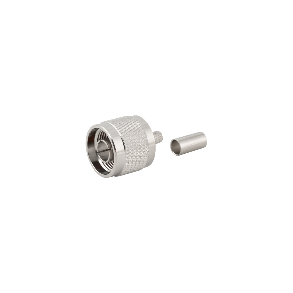 N-Type RF Coaxial Connectors for Flexible CableN-type connectors for flexible cable with crimp, clamp, or solder termination; useful where cable attachment and plating choices distinguish otherwise similar parts.View Product →
Mechanical Specifications and Installation Limits
Mechanical limits are the ones that fail months later, so treat them as design inputs rather than installation notes.
- Bend radius — a tight bend deforms the dielectric, shifts local impedance and can permanently raise attenuation.
- Mating cycles — precision interfaces such as 2.92 mm are rated for far fewer cycles than a BNC; a lab cable used as a daily patch lead will wear out.
- Torque — under-torqued SMA joints produce intermittent contact, over-torqued ones damage the dielectric.
- Temperature and jacket — outdoor and plenum routes need a jacket rating, and the connector's range can be narrower than the cable's.
- Dimensions — centre conductor, dielectric and outer diameter tolerances explain most “same size, does not fit” complaints.
Reading a Datasheet Without Being Misled
A specification is only usable when it states frequency, temperature, and whether the value is typical, maximum or guaranteed. Anything less belongs in an email, not a design file.
- Typical versus guaranteed: “typical” is a population average, while a guaranteed maximum is what a link budget needs.
- Length basis: dB/100 m and dB/100 ft differ by a factor of about 3.28, and mixing them overstates margin.
- Test conditions: a short sample measured with laboratory connectors will not match a terminated assembly with a bulkhead fitting.
- Frequency of record: a figure at 1 GHz says little about behaviour at 5.8 GHz.
- Assembly loss: add connector pairs, adapters and any protector before comparing two cable grades.
Matching Connectors, Adapters and Surge Protection
Every element between radio and antenna adds loss and a mismatch, so protecting margin usually means removing parts rather than upgrading cable.
Adapters are the hidden cost. One intertype adapter typically adds 0.1 to 0.3 dB plus another mating plane, and a chain of three can cost more than the difference between two cable grades. If a design needs N-to-SMA conversion at a panel, one adapter at the bulkhead beats two in free air, and a within-type adapter is usually preferable to a stack.
 N to SMA Inter-Type RF Coaxial Adapter50Ω N-to-SMA adapter in four gender combinations, supporting test, installation, and system integration between N feedlines and SMA-port components.View Product →
Surge protection sits in the same chain and deserves the same scrutiny: insertion loss across the working band, a defined clamping voltage, and a surge rating above the energy you expect. A protector that costs 0.5 dB but prevents a front-end replacement is a sound trade; one specified without a frequency range is not. The coaxial lightning protector range is organised by interface for exactly this reason — the protector must match the connector series, not merely the impedance.
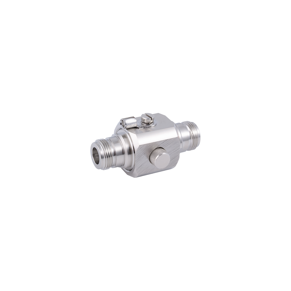 N-Type Coaxial Lightning Protector ManufacturerYangzhou Jingcheng Electronics Co., Ltd., a premier China N-Type Coaxial Lightning Protector Manufacturer and N-Type Coaxial Lightning Protector Factory , was founded ...View Product →
Frequently Asked Questions
What is the most important coaxial cable specification?
Impedance, because a mismatch cannot be corrected downstream. Once impedance is right, attenuation at the operating frequency becomes the deciding number.
Does cable length change the specifications?
It changes the totals, not the per-unit figures. Loss and delay scale with length; impedance, velocity factor and capacitance per metre do not. A 30 m run at 2.4 GHz in thin cable can lose well over 20 dB, so length belongs in the first calculation.
Can I use 75 Ω cable with a 50 Ω connector?
It will assemble, and short low-frequency runs may even work. At higher frequencies the impedance step at the joint produces a reflection that appears as poor return loss, pattern distortion or intermittent errors. Use the matching family, or accept the penalty knowingly.
Which attenuation figure belongs in a link budget?
The worst case at the highest frequency of interest, for the stated length, plus connector and adapter losses. Adding 10 to 20% margin for temperature and installation variation is normal practice.
How do I confirm a connector matches a cable?
Match three dimensions — centre conductor, dielectric diameter and outer diameter — plus the cable type. Interface series alone is never enough: an SMA for flexible cable and an SMA for semi-rigid cable share a mating face, not a body.
A Short Checklist Before You Order
Most specification failures trace back to a detail that was never written down, so put these five items into the purchase request.
- Impedance with its tolerance, stated explicitly for the chosen family.
- Attenuation as a guaranteed maximum at the operating frequency, with the length basis spelled out.
- Bend radius and torque limits checked against the real routing and the real tools.
- Interface series, cable type and plating confirmed against an assembly drawing, not a photo.
- Protector insertion loss and clamping voltage, if a protector is part of the run.
None of these checks takes long. The ones that get skipped are the ones that reappear later as a link that technically works but cannot be trusted.